Analysing behavioral data using clustering
Can we use clustering to find meaningful insights when zebrafish are faced with two competing threatening stimuli?
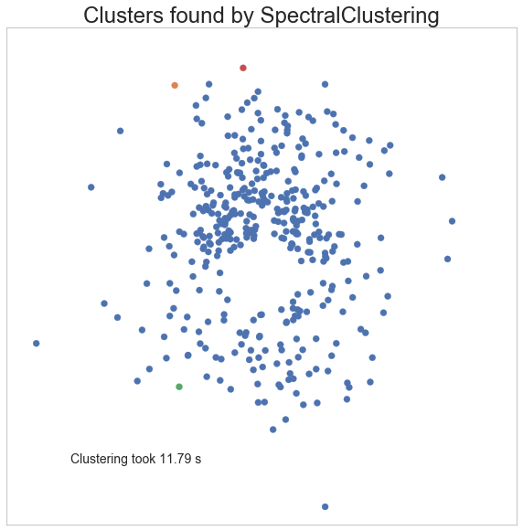
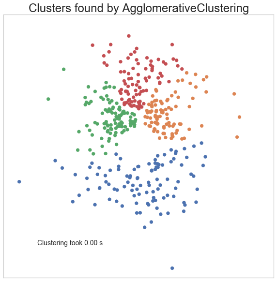
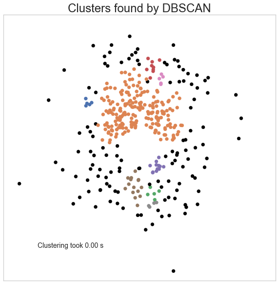
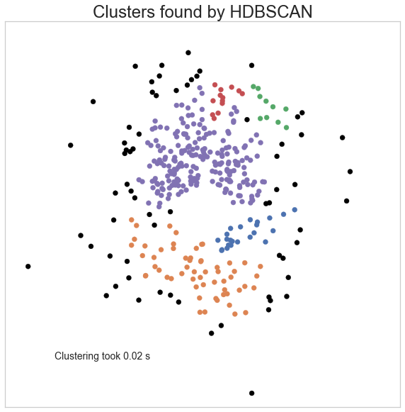
Answer: No. This approach does not reveal distinct response types.Clustering is NOT a good approach for this behavioral data. Boundaries seem arbitrary.
See below Notebook or Repository link
Trying out clustering on behavioral decisions of zebrafish when they are faced with two competing threatening stimuli. This data is related to the following publication: Neuronal circuitry for stimulus selection in the visual system.
Repository Link
import pandas as pd
import matplotlib.pyplot as plt
import numpy as np
import seaborn as sns
import scipy.stats as sta
from itertools import groupby
import os
import glob

%reload_ext autoreload
%autoreload 2
%matplotlib inline
import sys
print("Python version")
print (sys.version)
Python version
3.7.2 (default, Dec 29 2018, 00:00:04)
[Clang 4.0.1 (tags/RELEASE_401/final)]
Specify file containing behavioral data
df=pd.read_csv('MF319_competition_3_conditions_df_.csv', index_col=0)
df.head()
| animalID | c1 | c2 | condition | e | expAnimal | experiment | frame | frameCont | l | ... | yp2 | treatment | xOriginal | yOriginal | front | right | left | r | centerDist | lastStep | |
|---|---|---|---|---|---|---|---|---|---|---|---|---|---|---|---|---|---|---|---|---|---|
| 0 | 0.0 | 1.0 | 0.0 | 4 | 1.0 | 0.0 | 0.0 | 0.0 | 2800.0 | 0.0 | ... | 0.630044 | 0 | 235.0 | 430.0 | 0.0 | 0.0 | 0.0 | -0.000000 | 0.0 | 0.0 |
| 1 | 0.0 | 1.0 | 0.0 | 4 | 1.0 | 0.0 | 0.0 | 1.0 | 2801.0 | 0.0 | ... | 0.630044 | 0 | 235.0 | 430.0 | 0.0 | 0.0 | 0.0 | -0.000000 | 0.0 | 0.0 |
| 2 | 0.0 | 1.0 | 0.0 | 4 | 1.0 | 0.0 | 0.0 | 2.0 | 2802.0 | 0.0 | ... | 0.630044 | 0 | 234.0 | 430.0 | 1.0 | 0.0 | 1.0 | 1.834389 | 1.0 | 1.0 |
| 3 | 0.0 | 1.0 | 0.0 | 4 | 1.0 | 0.0 | 0.0 | 3.0 | 2803.0 | 0.0 | ... | 0.630044 | 0 | 234.0 | 430.0 | 1.0 | 0.0 | 1.0 | 1.834389 | 1.0 | 0.0 |
| 4 | 0.0 | 1.0 | 0.0 | 4 | 1.0 | 0.0 | 0.0 | 4.0 | 2804.0 | 0.0 | ... | 0.630044 | 0 | 234.0 | 430.0 | 1.0 | 0.0 | 1.0 | 1.834389 | 1.0 | 0.0 |
5 rows × 31 columns
df.columns
Index(['animalID', 'c1', 'c2', 'condition', 'e', 'expAnimal', 'experiment',
       'frame', 'frameCont', 'l', 'o', 's1', 's1b', 's2', 's2b', 'trial', 'x',
       'xp1', 'xp2', 'y', 'yp1', 'yp2', 'treatment', 'xOriginal', 'yOriginal',
       'front', 'right', 'left', 'r', 'centerDist', 'lastStep'],
      dtype='object')
df.condition.unique()
array([4, 7, 1])
df.trial.max()
300.0
#specify time limits for analysis, i.e. to exclude very late trials
first_trial=0
last_trial=300

#pull only trials within time limits
dfEarly=df[(df.trial<last_trial)&(df.trial>first_trial)]

#generate a unique ID from animalID and trial number
dfEarly.loc[:,'anTrial']=dfEarly.trial.values + dfEarly.animalID.values*dfEarly.trial.values.max()

# #only consider animals that moved by more than a threshold
ResponseThreshold=30  #should be  around 4mm according to calculations.

ind=(dfEarly.centerDist>=ResponseThreshold)&(dfEarly.frame<=dfEarly.frame.max())
d=dfEarly[ind]
last_frame_stim=15 #last frame for looming presentation for each tRial. End of expansion
#condition 1 is coNdition with right stimu only
#condition 4 is coNdition  with left stimu only
#condition 7 is coNdition with both stimuli (equal stim competition)


x_right_stim=d.x[(d.condition==1)&(d.frame==last_frame_stim)]
y_right_stim=d.y[(d.condition==1)&(d.frame==last_frame_stim)]
x_left_stim=d.x[(d.condition==4)&(d.frame==last_frame_stim)]
y_left_stim=d.y[(d.condition==4)&(d.frame==last_frame_stim)]
x_competition=d.x[(d.condition==7)&(d.frame==last_frame_stim)]
y_competition=d.y[(d.condition==7)&(d.frame==last_frame_stim)]


right_stim=np.stack([x_right_stim,y_right_stim])
left_stim=np.stack([x_left_stim,y_left_stim])
both_stim=np.stack([x_competition,y_competition])
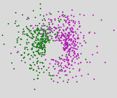
'''Condition with right or left stimuli alone'''

fig = plt.figure(figsize= (10, 10))
plt.scatter(right_stim[0],right_stim[1], color='g',label='right loom')
plt.scatter(left_stim[0],left_stim[1], color='m',label='left loom')
plt.legend(loc='upper right')
plt.xlim(-200,200)
plt.ylim(-200,200)
sns.despine()
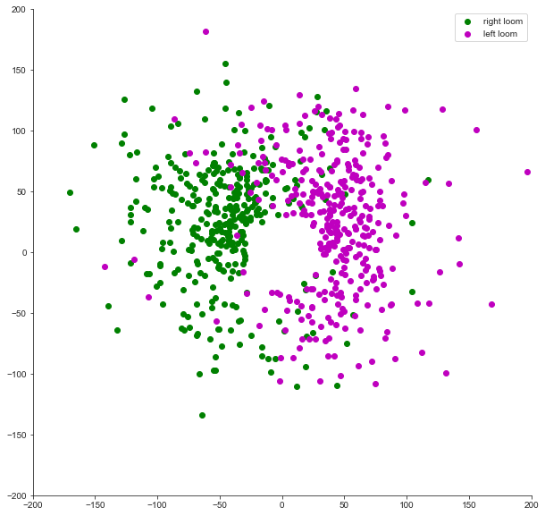
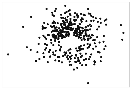
'''Condition with both stimuli'''

fig = plt.figure(figsize= (10, 10))
plt.scatter(both_stim[0],both_stim[1], color='k', label= 'Both stim')
plt.legend(loc='upper right')
plt.xlim(-200,200)
plt.ylim(-200,200)
sns.despine()
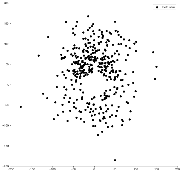
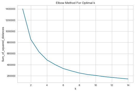
Trying KMeans clustering
Checking which K to use
from sklearn.cluster import KMeans
X=np.transpose(both_stim) #transpose to match what is expected for fit

Sum_of_squared_distances = []
K = range(1,15)
for k in K:
    km = KMeans(n_clusters=k)
    km = km.fit(X)
    Sum_of_squared_distances.append(km.inertia_)
plt.plot(K, Sum_of_squared_distances, 'bx-')
plt.xlabel('k')
plt.ylabel('Sum_of_squared_distances')
plt.title('Elbow Method For Optimal k')
plt.show()
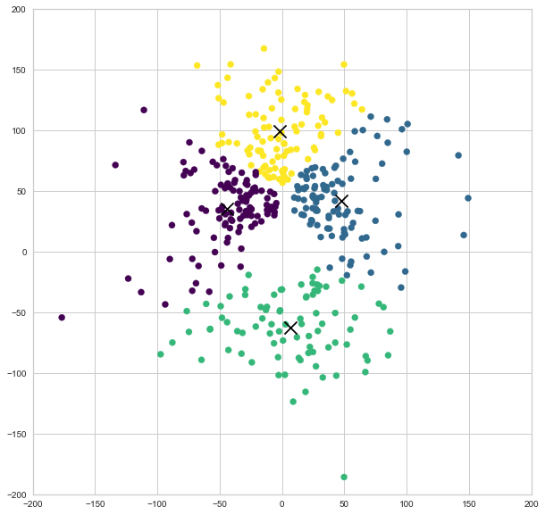
kmeans = KMeans(n_clusters=4)
kmeans.fit(X)
y_kmeans = kmeans.predict(X)

fig = plt.figure(figsize= (10, 10))
plt.scatter(X[:, 0], X[:, 1], c=y_kmeans, s=50, cmap='viridis')

centers = kmeans.cluster_centers_
plt.scatter(centers[:, 0], centers[:, 1], c='black', s=200, alpha=1, marker='x');


plt.xlim(-200,200)
plt.ylim(-200,200)
(-200, 200)
Testing Gaussian mixture model probability distribution
Based on https://jakevdp.github.io/PythonDataScienceHandbook/05.12-gaussian-mixtures.html
from sklearn import mixture
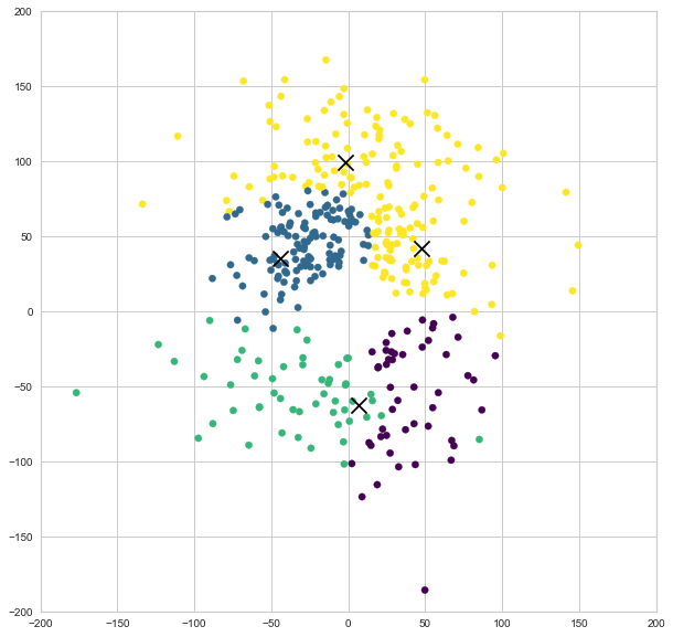
gmm = mixture.GaussianMixture(n_components=4).fit(X)
labels = gmm.predict(X)
fig = plt.figure(figsize= (10, 10))
plt.scatter(X[:, 0], X[:, 1], c=labels, s=40, cmap='viridis');
centers = kmeans.cluster_centers_
plt.scatter(centers[:, 0], centers[:, 1], c='black', s=200, alpha=1, marker='x');
plt.xlim(-200,200)
plt.ylim(-200,200)
(-200, 200)
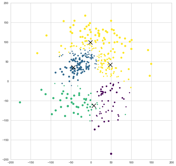
'''find probabilistic cluster assignments'''
probs = gmm.predict_proba(X)
print(probs[:5].round(3))

fig = plt.figure(figsize= (10, 10))
size = 50 * probs.max(1) ** 2  # square emphasizes differences
plt.scatter(X[:, 0], X[:, 1], c=labels, cmap='viridis', s=size);
centers = kmeans.cluster_centers_
plt.scatter(centers[:, 0], centers[:, 1], c='black', s=200, alpha=1, marker='x');
plt.legend
plt.xlim(-200,200)
plt.ylim(-200,200)
[[0.    0.464 0.    0.536]
 [0.    0.24  0.    0.76 ]
 [0.    0.89  0.    0.11 ]
 [0.003 0.    0.    0.997]
 [0.    0.247 0.    0.753]]


(-200, 200)
from sklearn.cluster import KMeans
X=np.transpose(right_stim) #transpose to match what is expected for fit

Sum_of_squared_distances = []
K = range(1,15)
for k in K:
    km = KMeans(n_clusters=k)
    km = km.fit(X)
    Sum_of_squared_distances.append(km.inertia_)
plt.plot(K, Sum_of_squared_distances, 'bx-')
plt.xlabel('k')
plt.ylabel('Sum_of_squared_distances')
plt.title('Elbow Method For Optimal k')
plt.show()
Comparing clustering methods in a systematic way
Based on https://hdbscan.readthedocs.io/en/latest/comparing_clustering_algorithms.html
X=np.transpose(equal_stim) #transpose to match what is expected for fit
data=X
plt.scatter(data.T[0], data.T[1], c='k')
frame = plt.gca()
frame.axes.get_xaxis().set_visible(False)
frame.axes.get_yaxis().set_visible(False)
def plot_clusters(data, algorithm, args, kwds, condition):
    start_time = time.time()
    labels = algorithm(*args, **kwds).fit_predict(data)
    end_time = time.time()
    palette = sns.color_palette('deep', np.unique(labels).max() + 1)
    colors = [palette[x] if x >= 0 else (0.0, 0.0, 0.0) for x in labels]
    fig = plt.figure(figsize= (10, 10))
    plt.scatter(data.T[0], data.T[1], c=colors)
    frame = plt.gca()
    frame.axes.get_xaxis().set_visible(False)
    frame.axes.get_yaxis().set_visible(False)
    plt.xlim(-200,200)
    plt.ylim(-200,200)
    plt.title('Clusters found by {}'.format(str(algorithm.__name__)), fontsize=24)
    plt.text(-150, -150, 'Clustering took {:.2f} s'.format(end_time - start_time), fontsize=14)
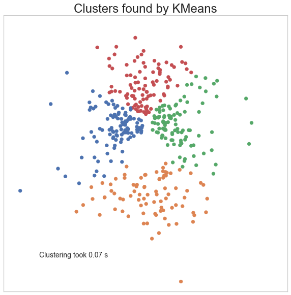
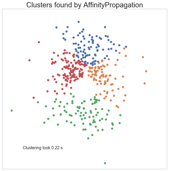
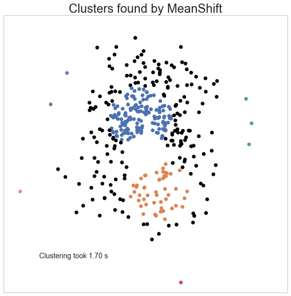
import sklearn.cluster as cluster
import time
plot_clusters(data, cluster.KMeans, (), {'n_clusters':4},'equal_stim')
plot_clusters(data, cluster.AffinityPropagation, (),\
              {'preference':-190000, 'damping':.95},'equal_stim')
plot_clusters(data, cluster.MeanShift, (45,), {'cluster_all':False},'equal_stim')
plot_clusters(data, cluster.SpectralClustering, (), {'n_clusters':4},'equal_stim')
/Users/fernandes/anaconda3/lib/python3.7/site-packages/sklearn/manifold/_spectral_embedding.py:236: UserWarning: Graph is not fully connected, spectral embedding may not work as expected.
  warnings.warn("Graph is not fully connected, spectral embedding"
plot_clusters(data, cluster.AgglomerativeClustering, (), {'n_clusters':4, 'linkage':'ward'},'equal_stim')
plot_clusters(data, cluster.DBSCAN, (), {'eps':12},'equal_stim')
import hdbscan
plot_clusters(data, hdbscan.HDBSCAN, (),{'min_cluster_size':8, 'min_samples':1},'equal_stim')
Try hierarchical clustering
from scipy.cluster.hierarchy import linkage, dendrogram
samples = X

"""
Perform hierarchical clustering on samples using the
linkage() function with the method='complete' keyword argument.
Assign the result to mergings.
"""
Z= linkage(samples, method='ward')
from matplotlib.pyplot import cm
from scipy.cluster import hierarchy
import matplotlib as mpl
"""
Plot a dendrogram using the dendrogram() function on mergings,
specifying the keyword arguments labels=varieties, leaf_rotation=90,
and leaf_font_size=6.
"""
cut=400
fig = plt.figure(figsize= (15, 15))

hierarchy.set_link_color_palette(['g', 'r', 'c', 'm', 'y', 'k'])


den=dendrogram(Z,
           leaf_rotation=90,
           leaf_font_size=6,
           color_threshold=cut,)   #define link color func using fcluster ids
#            truncate_mode='lastp',# show only the last p merged clusters
#            p=50) # show only the last p merged clusters

# print(den['leaves'], den['color_list'])
plt.gcf()
plt.axis('off')
plt.axhline(y=cut, color='k', linestyle='--')
<matplotlib.lines.Line2D at 0x1a30899748>

from scipy.cluster.hierarchy import ward, fcluster
cluster_id=fcluster(Z, t=cut, criterion='distance')
cluster_id=cluster_id-1 #cluster_id is relative to samples and is index -1
cluster_id
array([2, 2, 2, 4, 2, 4, 3, 1, 1, 3, 1, 2, 3, 3, 2, 4, 1, 3, 3, 3, 0, 2,
       2, 4, 1, 4, 3, 4, 3, 3, 2, 3, 4, 3, 0, 0, 2, 3, 3, 2, 0, 3, 2, 2,
       3, 4, 2, 4, 2, 4, 0, 2, 3, 2, 0, 2, 4, 3, 0, 2, 2, 2, 4, 3, 1, 2,
       2, 0, 0, 0, 2, 2, 2, 1, 2, 2, 1, 3, 2, 4, 2, 4, 0, 0, 2, 2, 1, 1,
       0, 4, 3, 1, 3, 3, 3, 3, 3, 3, 3, 3, 3, 2, 1, 2, 4, 0, 0, 3, 3, 3,
       3, 2, 3, 3, 3, 4, 3, 4, 4, 4, 1, 1, 2, 1, 2, 3, 3, 4, 4, 2, 1, 1,
       1, 0, 1, 3, 3, 1, 1, 4, 4, 4, 4, 3, 4, 2, 4, 0, 1, 1, 2, 3, 3, 1,
       3, 1, 1, 0, 4, 1, 0, 3, 0, 3, 0, 1, 0, 2, 4, 2, 2, 0, 0, 3, 2, 1,
       2, 2, 4, 1, 0, 3, 4, 4, 2, 3, 0, 3, 4, 2, 3, 3, 3, 3, 4, 3, 4, 0,
       0, 4, 4, 4, 3, 4, 3, 2, 4, 3, 4, 3, 4, 1, 3, 3, 2, 0, 1, 2, 2, 0,
       2, 3, 4, 2, 2, 4, 3, 2, 4, 0, 4, 4, 2, 4, 0, 1, 4, 4, 2, 3, 3, 4,
       4, 1, 2, 2, 2, 1, 2, 3, 1, 1, 4, 0, 1, 1, 1, 4, 1, 0, 4, 4, 4, 1,
       4, 1, 4, 0, 0, 0, 1, 1, 2, 2, 2, 1, 3, 2, 2, 0, 3, 4, 3, 3, 2, 3,
       1, 3, 2, 2, 4, 2, 3, 4, 3, 2, 2, 2, 4, 4, 2, 1, 3, 4, 4, 1, 1, 3,
       4, 4, 3, 0, 4, 4, 3, 1, 4, 0, 4, 3, 2, 4, 3, 3, 4, 2, 2, 4, 1, 4,
       4, 1, 3, 4, 0, 0, 3, 2, 2, 2, 0, 2, 2, 0, 2, 1, 3, 4, 2, 4, 4, 2,
       4, 4, 4, 3, 4, 2, 2, 0, 2, 2, 1, 2, 4, 4, 2, 4, 2, 2, 2, 4, 4, 4,
       2, 2, 3, 2, 1, 4, 2, 1, 2, 2, 2, 1], dtype=int32)
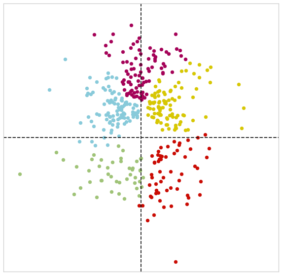
fig = plt.figure(figsize= (10, 10))
plt.scatter(samples[cluster_id ==0,0], samples[cluster_id == 0,1], s=50, c='g')
plt.scatter(samples[cluster_id==1,0], samples[cluster_id== 1,1], s=50, c='r')
plt.scatter(samples[cluster_id ==2,0], samples[cluster_id == 2,1], s=50, c='c')
plt.scatter(samples[cluster_id ==3,0], samples[cluster_id == 3,1], s=50, c='m')
plt.scatter(samples[cluster_id ==4,0], samples[cluster_id == 4,1], s=50, c='y')
frame = plt.gca()
plt.legend
plt.xlim(-200,200)
plt.ylim(-200,200)
plt.vlines(0,-200,200, linestyles="dashed")
plt.hlines(0,-200,200, linestyles="dashed")

frame.axes.get_xaxis().set_visible(False)
frame.axes.get_yaxis().set_visible(False)
left=samples[cluster_id ==2].shape[0]
back=samples[cluster_id ==0].shape[0]+samples[cluster_id ==1].shape[0]
right=samples[cluster_id ==4].shape[0]
front=samples[cluster_id ==3].shape[0]
total_responses=np.sum([left,back,right,front])
print ('% left', left/total_responses*100)
print ('% right', right/total_responses*100)
print ('% front', front/total_responses*100)

print ('% left + right together', (left+right)/total_responses*100)
print ('% back together', back/total_responses*100)
% left 26.42487046632124
% right 24.093264248704664
% front 22.797927461139896
% left + right together 50.51813471502591
% back together 26.683937823834196
Conclusions:
Clustering is NOT a good approach for this behavioral data. Boundaries seem arbitrary. Need to model the data in a continuous space (circular data)
Miguel Fernandes
Senior Data Scientist
My interests include neuroscience, education, artificial intelligence and genetics.